ultrasphere package
- class ultrasphere.BranchingType(*values)[source]
Bases:
StrEnumThe branching types of the nodes in a rooted tree representing the coordinates.
(Vilenkin’s method of trees)
- A = 'a'
- B = 'b'
- BP = "b'"
- C = 'c'
- class ultrasphere.SphericalCoordinates(tree: DiGraph, /)[source]
Bases:
GenericStores the spherical coordinates using the method of trees by Vilenkin.
Examples
>>> import ultrasphere as us
>>> c = us.create_standard(3)
>>> c
SphericalCoordinates(bba)
>>> c.s_nodes
['theta0', 'theta1', 'theta2']
>>> c.c_nodes
[0, 1, 2, 3]
>>> c.branching_types
{'theta0': <BranchingType.B: 'b'>, 'theta1': <BranchingType.B: 'b'>, 'theta2': <BranchingType.A: 'a'>}
>>> c.cos_edges
[('theta0', 0), ('theta1', 1), ('theta2', 2)]
>>> c.sin_edges
[('theta0', 'theta1'), ('theta1', 'theta2'), ('theta2', 3)]
>>> c.S
{3: nan, 2: nan, 'theta2': 0, 1: nan, 'theta1': 1, 0: nan, 'theta0': 2}
- G: DiGraph
The rooted tree representing the coordinates.
- S: Mapping[TSpherical, int]
The number of non-leaf descendants for each spherical node.
- branching_types: Mapping[TSpherical, BranchingType]
The branching types of each node.
- property branching_types_expression: Sequence[BranchingType]
The branching types.
Examples
>>> import ultrasphere as us
>>> us.create_standard(2).branching_types_expression
[<BranchingType.B: 'b'>, <BranchingType.A: 'a'>]
- property branching_types_expression_str: str
The branching types as a string.
Examples
>>> import ultrasphere as us
>>> us.create_standard(3).branching_types_expression_str
'bba'
- property c_ndim: int
The number of Cartesian dimensions.
Examples
>>> import ultrasphere as us
>>> us.create_standard(3).c_ndim
4
- c_nodes: Sequence
The Cartesian nodes.
- cos_edges: Sequence[tuple[TSpherical, TCartesian | TSpherical]]
The edges with type ‘cos’.
- from_cartesian(cartesian: Mapping[TCartesian, Array], /) Mapping[TSpherical | Literal['r'], Array][source]
Convert the Cartesian coordinates to the spherical coordinates.
- Parameters:
cartesian (Mapping[TCartesian, Array]) – The Cartesian coordinates.
- Returns:
The spherical coordinates.
- Return type:
Array
Examples
>>> import ultrasphere as us
>>> from array_api_compat import numpy as np
>>> c = us.create_spherical()
>>> s = c.from_cartesian(np.asarray([1.0, 2.0, 3.0]))
>>> {k: np.round(s[k], 6) for k in c.s_nodes + ["r"]}
{'theta': np.float64(0.640522), 'phi': np.float64(1.107149), 'r': np.float64(3.741657)}
- property is_c_keys_range: bool
Whether the Cartesian keys are 0, 1, …, c_ndim - 1.
- property is_s_keys_range: bool
Whether the spherical keys are 0, 1, …, s_ndim - 1.
- jacobian(spherical: Mapping[TSpherical | Literal['r'], Array] | Mapping[TSpherical, Array], /) Array[source]
Calculate the Jacobian of the spherical coordinates.
- Parameters:
spherical (Mapping[TSpherical, Array]) – The spherical coordinates.
- Returns:
The Jacobian of the spherical coordinates.
- Return type:
Array
- property root: Any
The root node.
Examples
>>> import ultrasphere as us
>>> us.create_standard(3).root
'theta0'
- property root_index: int
The index of the root node.
- property s_ndim: int
The number of spherical dimensions.
Examples
>>> import ultrasphere as us
>>> us.create_standard(3).s_ndim
3
- s_nodes: Sequence
The spherical nodes.
- sin_edges: Sequence[tuple[TSpherical, TCartesian | TSpherical]]
The edges with type ‘sin’.
- surface_area(r: float = 1) float[source]
The surface area of the unit sphere.
\[|\mathbb{S}^{d-1}| = \frac{2 \pi^{d/2}}{\Gamma(d/2)} r^{d-1}\]- Parameters:
r (float, optional) – The radius, by default 1
- Returns:
The surface area.
- Return type:
float
Examples
>>> import ultrasphere as us
>>> from array_api_compat import numpy as np
>>> np.round(us.create_standard(2).surface_area(), 6)
np.float64(12.566371)
- to_cartesian(spherical: Mapping[TSpherical | Literal['r'], Array] | Mapping[TSpherical, Array], /, *, as_array: Literal[False] = False) Mapping[TCartesian, Array][source]
- to_cartesian(spherical: Mapping[TSpherical | Literal['r'], Array] | Mapping[TSpherical, Array], /, *, as_array: Literal[True] = False) Array
Convert the spherical coordinates to the Cartesian coordinates.
- Parameters:
spherical (Mapping[TSpherical, Array]) – The spherical coordinates.
as_array (bool, optional) – Whether to return as an array, by default False
- Returns:
The Cartesian coordinates.
- Return type:
Array
Examples
>>> import ultrasphere as us
>>> from array_api_compat import numpy as np
>>> c = us.create_spherical()
>>> e = c.to_cartesian({"theta": np.float64(0.640522), "phi": np.float64(1.107149), "r": np.float64(3.741657)})
>>> {k: np.round(e[k], 5) for k in c.c_nodes}
{0: np.float64(1.0), 1: np.float64(2.0), 2: np.float64(3.0)}
- volume(r: float = 1) float[source]
The volume of the unit sphere.
\[\Upsilon_d = \frac{\pi^{d/2}}{\Gamma(d/2 + 1)} r^d\]- Parameters:
r (float, optional) – The radius, by default 1
- Returns:
The volume.
- Return type:
float
References
McLean, W. (2000). Strongly Elliptic Systems and Boundary Integral Equations. p.247 (Upsilon_n)
Examples
>>> import ultrasphere as us
>>> from array_api_compat import numpy as np
>>> np.round(us.create_standard(2).volume(), 6)
np.float64(4.18879)
- ultrasphere.create_from_branching_types(branching_types: str | Sequence[BranchingType]) SphericalCoordinates[Any, Any][source]
Spherical coordinates from branching types.
- Parameters:
branching_types (str | Sequence[BranchingType]) – The branching types. e.g. “ba” for standard spherical coordinates.
- Returns:
The spherical coordinates.
- Return type:
- ultrasphere.create_hopf(q: int) SphericalCoordinates[Any, Any][source]
Hopf coordinates.
- Parameters:
q (int) – Where 2^q = c.c_ndim.
- Returns:
The Hopf coordinates.
- Return type:
Examples
>>> c = create_hopf(3)
>>> c
SphericalCoordinates(ccaacaa)
>>> c.s_nodes
['theta0', 'theta1', 'theta2', 'theta3', 'theta4', 'theta5', 'theta6']
>>> c.c_nodes
[0, 1, 2, 3, 4, 5, 6, 7]
- ultrasphere.create_polar() SphericalCoordinates[Literal['phi'], Literal[0, 1]][source]
Polar coordinates.
\[\begin{split}x_0 &= r \cos(\phi) \\ x_1 &= r \sin(\phi)\end{split}\]- Returns:
The polar coordinates.
- Return type:
Examples
>>> c = create_polar()
>>> c
SphericalCoordinates(a)
>>> c.s_nodes
['phi']
>>> c.c_nodes
[0, 1]
- ultrasphere.create_random(s_ndim: int, *, rng: Generator | None = None) SphericalCoordinates[Any, Any][source]
Get a random spherical coordinates.
- Parameters:
s_ndim (int) – The number of spherical dimensions.
rng (np.random.Generator | None, optional) – The random number generator, by default None
- Returns:
The random spherical coordinates.
- Return type:
Examples
>>> from array_api_compat import numpy as np
>>> rng = np.random.default_rng(0)
>>> c = create_random(5, rng=rng)
>>> c
SphericalCoordinates(bcb'aa)
>>> c.s_nodes
['theta0', 'theta1', 'theta2', 'theta3', 'theta4']
>>> c.c_nodes
[0, 1, 2, 3, 4, 5]
- ultrasphere.create_spherical() SphericalCoordinates[Literal['theta', 'phi'], Literal[0, 1, 2]][source]
Spherical coordinates.
\[\begin{split}x_0 &= r \sin(\theta) \cos(\phi) \\ x_1 &= r \sin(\theta) \sin(\phi) \\ x_2 &= r \cos(\theta)\end{split}\]- Returns:
The spherical coordinates.
- Return type:
Examples
>>> c = create_spherical()
>>> c
SphericalCoordinates(ba)
>>> c.s_nodes
['theta', 'phi']
>>> c.c_nodes
[0, 1, 2]
- ultrasphere.create_standard(s_ndim: int) SphericalCoordinates[Any, Any][source]
Standard spherical coordinates.
\[\begin{split}x_0 &= \cos(\theta_0) \\ x_1 &= \sin(\theta_0) \cos(\theta_1) \\ x_2 &= \sin(\theta_0) \sin(\theta_1) \cos(\theta_2) \\ x_3 &= \sin(\theta_0) \sin(\theta_1) \sin(\theta_2) \cos(\theta_3) \\ &\vdots \\\end{split}\]- Parameters:
s_ndim (int) – The number of spherical dimensions.
- Returns:
The standard coordinates.
- Return type:
Examples
>>> c = create_standard(4)
>>> c
SphericalCoordinates(bbba)
>>> c.s_nodes
['theta0', 'theta1', 'theta2', 'theta3']
>>> c.c_nodes
[0, 1, 2, 3, 4]
- ultrasphere.create_standard_prime(s_ndim: int) SphericalCoordinates[Any, Any][source]
Standard prime spherical coordinates.
\[\begin{split}x_0 &= \sin(\theta_0) \\ x_1 &= \cos(\theta_0) \sin(\theta_1) \\ x_2 &= \cos(\theta_0) \cos(\theta_1) \sin(\theta_2) \\ x_3 &= \cos(\theta_0) \cos(\theta_1) \cos(\theta_2) \sin(\theta_3) \\ &\vdots \\\end{split}\]- Parameters:
s_ndim (int) – The number of spherical dimensions.
- Returns:
The standard prime coordinates.
- Return type:
Examples
>>> c = create_standard_prime(4)
>>> c
SphericalCoordinates(b'b'b'a)
>>> c.s_nodes
['theta0', 'theta1', 'theta2', 'theta3']
>>> c.c_nodes
[0, 1, 2, 3, 4]
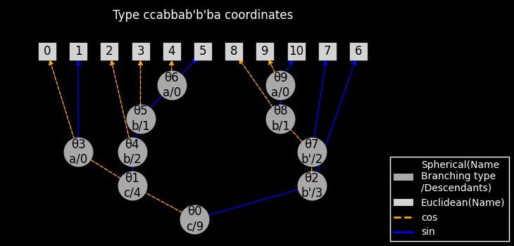
- ultrasphere.draw(c: SphericalCoordinates[TSpherical, TCartesian], root_bottom: bool = True, ax: Axes | None = None) tuple[float, float][source]
Nicely draw the rooted tree representing the coordinates using matplotlib.
- Parameters:
root_bottom (bool, optional) – Whether to draw the root at the bottom, by default True
- Returns:
The recommended width and height of the figure (in inches).
- Return type:
tuple[float, float]
Example
>>> import ultrasphere as us
>>> c = us.create_from_branching_types("ccabbab'b'ba")
>>> us.draw(c)
(6.5, 3.5)
- ultrasphere.fundamental_solution(d: TArray, z: TArray, k: TArray, derivative: bool = False) TArray[source]
Fundamental solution of the Helmholtz equation in d dimensions.
- Parameters:
d (TArray) – The dimension of the space.
z (TArray) – The argument of the fundamental solution of shape (…, d (coordinates)).
k (TArray) – The wave number.
derivative (bool, optional) – Whether to compute the derivative of the fundamental solution, by default False
- Returns:
The fundamental solution of the Helmholtz equation of shape (…,).
- Return type:
TArray
- ultrasphere.get_child(G: DiGraph, node: Any, type: Literal['cos', 'sin'], /) Any[source]
Get the child node of the given type in a rooted tree representing the coordinates.
- Parameters:
G (nx.DiGraph) – A rooted tree representing the coordinates.
node (Any) – The node to get the child.
type (COSSIN) – The type of the child._description_
- Raises:
ValueError – If the node has no child of the given type. If the node has multiple children of the given type.
- ultrasphere.get_parent(G: DiGraph, node: Any, /) Any | None[source]
Get the parent node in a rooted tree representing the coordinates.
- Parameters:
G (nx.DiGraph) – A rooted tree representing the coordinates.
node (Any) – The node to get the parent.
- Returns:
The parent node if exists, otherwise None.
- Return type:
Any
- Raises:
ValueError – If the node has multiple parents.
- ultrasphere.integrate(c: SphericalCoordinates[TSpherical, TCartesian], f: Callable[[Mapping[TSpherical, Array]], Mapping[TSpherical, Array]] | Mapping[TSpherical, Array], does_f_support_separation_of_variables: Literal[True], n: int, *, xp: ArrayNamespaceFull, device: Any | None = None, dtype: Any | None = None) Mapping[TSpherical, Array][source]
- ultrasphere.integrate(c: SphericalCoordinates[TSpherical, TCartesian], f: Callable[[Mapping[TSpherical, Array]], Array] | Array, does_f_support_separation_of_variables: Literal[False], n: int, *, xp: ArrayNamespaceFull, device: Any | None = None, dtype: Any | None = None) Array
Integrate the function over the hypersphere.
\[\int_{\mathbb{S}^{d-1}} f d\omega^{d-1}\]- Parameters:
f (Callable[ [Mapping[TSpherical, Array]], Mapping[TSpherical, Array] | Array, ] | Mapping[TSpherical, Array] | Array # noqa: E501) –
The function to integrate or the values of the function.
If mapping, the separated parts of the function for each spherical coordinate.
If mapping, the shapes do not need to be broadcastable.
If function, if does_f_support_separation_of_variables is True, 1D array of integration points are passed, and extra axis should be added to the last dimension.
If function, if does_f_support_separation_of_variables is False,
c.s_ndim-D array of integration points are passed, and extra axis should be added to the last dimension.does_f_support_separation_of_variables (bool) – Whether the function supports separation of variables. This could significantly reduce the computational cost.
n (int) – The number of roots.
device (Any, optional) – The device, by default None
dtype (Any, optional) – The data type, by default None
- Returns:
The integrated value. Has the same shape as the return values of f or the values of f.
- Return type:
Array | Mapping[TSpherical, Array]
Example
>>> from array_api_compat import numpy as np
>>> import ultrasphere as us
>>> c = us.create_spherical()
>>> f = lambda spherical: spherical["theta"] ** 2 * spherical["phi"]
>>> np.round(us.integrate(
...     c,
...     f,
...     False, # does not support separation of variables
...     10, # number of quadrature points
...     xp=np # the array namespace
... ), 5)
np.float64(110.02621)
- ultrasphere.potential_coef(n: TArray, d: TArray, k: TArray, /, *, x_abs: TArray, y_abs: TArray, x_abs_derivative: bool | None = None, y_abs_derivative: bool | None = None, derivative: Literal['S', 'D', 'D*', 'N'] | None = None, limit: Literal[False, 'x_larger', 'y_larger', 'warn'] = 'warn', for_func: Literal['harmonics', 'solution'] = 'harmonics') Array[source]
The coefficients for layer potentials.
The coefficients for single-layer or double-layer potential for hyperspherical harmonics with homogeneous degree (maximum quantum number) n.
y is the integral variable.
\[r \mathbb{S}^{d-1} := \{ x \in \mathbb{R}^d : \left|x\right| = r \}\]\[\begin{split}\forall d \in \mathbb{N} \setminus \{1\}. \forall x_a, y_a \in (0, \infty). \forall T \in \{S_{y_a \mathbb{S}^{d-1}}, D_{y_a \mathbb{S}^{d-1}}, D^*_{y_a \mathbb{S}^{d-1}}, N_{y_a \mathbb{S}^{d-1}}\}. \\ \forall x \in x_a \mathbb{S}^{d-1}. \forall n \in \mathbb{N}_0. \forall Y_n \in \mathcal{H}(\mathbb{S}^{d-1}). \\ T Y_n \left(\frac{x}{x_a}\right) = \text{potential_coef}(T) Y_n \left(\frac{x}{x_a}\right)\end{split}\]- Parameters:
n (TArray) – The homogeneous degree of the hyperspherical harmonics. (maximum quantum number)
d (TArray) – The dimension of the hypersphere.
k (TArray) – The wavenumber.
x_abs (TArray) – The distance from the origin O to the point x.
y_abs (TArray) – The radius of the hypersphere.
x_abs_derivative (bool | None, optional) – Whether the derivative is taken with respect to x_abs, by default False.
y_abs_derivative (bool | None, optional) – Whether the derivative is taken with respect to y_abs, by default False.
derivative (Literal["S", "D", "D*", "N"] | None, optional) –
The shorthand for the derivative. Note that the integral variable is y.
”S” <=> x_abs_derivative = False, y_abs_derivative = False
”D” <=> x_abs_derivative = False, y_abs_derivative = True
”D*” <=> x_abs_derivative = True, y_abs_derivative = False
”N” <=> x_abs_derivative = True, y_abs_derivative = True
limit (Literal[False, "x_larger", "y_larger"], optional) – Whether to return the directional derivative of the potential with respect to x to the x/|x| direction, by default False.
for_func (Literal["harmonics", "solution"], optional) – Whether the coefficient is for the harmonics or the suitable (singular if outer, regular if inner) elementary solution, by default “harmonics”.
- Returns:
The coefficient for the potential integrated by y.
- Return type:
Array
References
McLean, W. (2000). Strongly Elliptic Systems and Boundary Integral Equations. p.285
- ultrasphere.random_ball(c: SphericalCoordinates[TSpherical, TCartesian], *, shape: Sequence[int], xp: ArrayNamespaceFull, device: Any | None = None, dtype: Any | None = None, type: Literal['uniform'] = 'uniform', rng: Generator | None = None, surface: bool = False) Array[source]
- ultrasphere.random_ball(c: SphericalCoordinates[TSpherical, TCartesian], *, shape: Sequence[int], xp: ArrayNamespaceFull, device: Any | None = None, dtype: Any | None = None, type: Literal['spherical'] = 'uniform', rng: Generator | None = None, surface: Literal[False] = False) Mapping[TSpherical | Literal['r'], Array]
- ultrasphere.random_ball(c: SphericalCoordinates[TSpherical, TCartesian], *, shape: Sequence[int], xp: ArrayNamespaceFull, device: Any | None = None, dtype: Any | None = None, type: Literal['spherical'] = 'uniform', rng: Generator | None = None, surface: Literal[True] = False) Mapping[TSpherical, Array]
Generate random points in the unit ball / sphere.
- Parameters:
shape (Sequence[int]) – The shape of the random points.
device (Any | None, optional) – The device, by default None
dtype (Any | None, optional) – The dtype, by default None
type (Literal["uniform", "spherical"], optional) – The type of the random points, by default “uniform” If “uniform”, the random points are uniformly distributed on the sphere. If “spherical”, each spherical coordinate (and radius if surface=False) is uniformly distributed.
rng (np.random.Generator | None, optional) – The random number generator, by default None
surface (bool, optional) – Whether to generate random points on the surface of the sphere or inside the sphere, by default False
- Returns:
The random points.
- Return type:
Mapping[TSpherical, Array] | Array | Mapping[TSpherical | Literal[“r”], Array]
References
Barthe, F., Guédon, O., Mendelson, S., & Naor, A. (2005). A probabilistic approach to the geometry of the ? P n -ball. The Annals of Probability, 33. https://doi.org/10.1214/009117904000000874
Examples
>>> from array_api_compat import numpy as xp
>>> import ultrasphere as us
>>> c = us.create_standard(4)
>>> rng = np.random.default_rng(0)
>>> points_ball = random_ball(c, shape=(2,), xp=xp, rng=rng)
>>> points_ball
array([[ 0.04083225, -0.08099814],
       [ 0.20798418,  0.06431795],
       [-0.17396442,  0.22170665],
       [ 0.4234881 ,  0.58068866],
       [-0.22854562, -0.77587443]])
>>> xp.linalg.vector_norm(points_ball, axis=0)
array([0.55386242, 0.99951577])
>>> points_sphere = random_ball(c, shape=(2,), xp=xp, rng=rng, surface=True)
>>> points_sphere
array([[-0.85238384, -0.11470655],
       [-0.45676572, -0.38390797],
       [-0.19953179, -0.16582762],
       [ 0.15090863,  0.54656157],
       [-0.04712233,  0.71639984]])
>>> xp.linalg.vector_norm(points_sphere, axis=0)
array([1., 1.])
- ultrasphere.roots(c: SphericalCoordinates[TSpherical, TCartesian], n: int, *, expand_dims_x: bool, expand_dims_w: bool = False, device: Any | None = None, dtype: Any | None = None, xp: ArrayNamespaceFull) tuple[Mapping[TSpherical, Array], Mapping[TSpherical, Array]][source]
Gauss-Jacobi quadrature roots and weights.
\[\int_\mathbb{S}^{d-1} f d\omega^{d-1} \approx \sum_{(\theta_1, w_1)} w_1 \cdots \sum_{(\theta_{d-1}, w_{d-1})} w_{d-1} f(\theta_1, \ldots, \theta_{d-1})\]- Parameters:
n (int) – The number of roots.
expand_dims_x (bool) – Whether to expand dimensions of the roots, by default False
expand_dims_w (bool, optional) – Whether to expand dimensions of the weights, by default False
device (Any, optional) – The device, by default None
dtype (Any, optional) – The data type, by default None
- Returns:
roots and weights
- Return type:
tuple[Mapping[TSpherical, Array], Mapping[TSpherical, Array]]
- Raises:
ValueError – If the branching type is invalid.
Example
>>> from array_api_compat import numpy as np
>>> import ultrasphere as us
>>> c = us.create_spherical()
>>> xs, ws = us.roots(c, 5, expand_dims_x=True, expand_dims_w=True, xp=np)
>>> xs
{'theta': array([[2.7049577 ],
       [2.13941585],
       [1.57079633],
       [1.0021768 ],
       [0.43663495]]), 'phi': array([[0.        , 0.62831853, 1.25663706, 1.88495559, 2.51327412,
        3.14159265, 3.76991118, 4.39822972, 5.02654825, 5.65486678]])}
>>> ws
{'theta': array([[0.23692689],
       [0.47862867],
       [0.56888889],
       [0.47862867],
       [0.23692689]]), 'phi': array([[0.62831853, 0.62831853, 0.62831853, 0.62831853, 0.62831853,
        0.62831853, 0.62831853, 0.62831853, 0.62831853, 0.62831853]])}
- ultrasphere.shn1(v: TArray, d: TArray, z: TArray, derivative: bool = False) TArray[source]
Hyperspherical Hankel function of the first kind.
\[h_v^{(1)(d)} (z) = \sqrt{\frac{\pi}{2}} \frac{H^{(1)}_{v + d/2 - 1}(z)}{z^{d/2 - 1}}\]- Parameters:
v (TArray) – The degree of the hyperspherical Hankel function.
d (TArray) – The dimension of the hypersphere.
z (TArray) – The argument of the hyperspherical Hankel function.
derivative (bool, optional) – Whether to compute the derivative of the hyperspherical Hankel function, by default False
- Returns:
The hyperspherical Hankel function of the first kind.
- Return type:
Array
- ultrasphere.shn2(v: TArray, d: TArray, z: TArray, derivative: bool = False) TArray[source]
Hyperspherical Hankel function of the second kind.
\[h_v^{(2)(d)} (z) = \sqrt{\frac{\pi}{2}} \frac{H^{(2)}_{v + d/2 - 1}(z)}{z^{d/2 - 1}}\]- Parameters:
v (TArray) – The degree of the hyperspherical Hankel function.
d (TArray) – The dimension of the hypersphere.
z (TArray) – The argument of the hyperspherical Hankel function.
derivative (bool, optional) – Whether to compute the derivative of the hyperspherical Hankel function, by default False
- Returns:
The hyperspherical Hankel function of the second kind.
- Return type:
Array
- ultrasphere.sjv(v: TArray, d: TArray, z: TArray, derivative: bool = False) TArray[source]
Hyperspherical Bessel function of the first kind.
\[j_v^{(d)} (z) = \sqrt{\frac{\pi}{2}} \frac{J_{v + d/2 - 1}(z)}{z^{d/2 - 1}}\]- Parameters:
v (TArray) – The degree of the hyperspherical Bessel function.
d (TArray) – The dimension of the hypersphere.
z (TArray) – The argument of the hyperspherical Bessel function.
derivative (bool, optional) – Whether to compute the derivative of the hyperspherical Bessel function, by default False
- Returns:
The hyperspherical Bessel function of the first kind.
- Return type:
Array
References
McLean, W. (2000). Strongly Elliptic Systems and Boundary Integral Equations. p.279
- ultrasphere.syv(v: TArray, d: TArray, z: TArray, derivative: bool = False) TArray[source]
Hyperspherical Bessel function of the second kind.
\[y_v^{(d)} (z) = \sqrt{\frac{\pi}{2}} \frac{Y_{v + d/2 - 1}(z)}{z^{d/2 - 1}}\]- Parameters:
v (TArray) – The degree of the hyperspherical Bessel function.
d (TArray) – The dimension of the hypersphere.
z (TArray) – The argument of the hyperspherical Bessel function.
derivative (bool, optional) – Whether to compute the derivative of the hyperspherical Bessel function, by default False
- Returns:
The hyperspherical Bessel function of the second kind.
- Return type:
Array
References
McLean, W. (2000). Strongly Elliptic Systems and Boundary Integral Equations. p.279
- ultrasphere.szv(v: TArray, d: TArray, z: TArray, type: Literal['j', 'y', 'h1', 'h2'], derivative: bool = False) TArray[source]
Utility function to compute hyperspherical functions.
\[f_v^{(d)} (z) = \sqrt{\frac{\pi}{2}} \frac{F_{v + d/2 - 1}(z)}{z^{d/2 - 1}}\]- Parameters:
v (TArray) – The degree of the hyperspherical Hankel function.
d (TArray) – The dimension of the hypersphere.
z (TArray) – The argument of the hyperspherical Hankel function.
type (Literal["j", "y", "h1", "h2"]) – The type of the hyperspherical function.
derivative (bool, optional) – Whether to compute the derivative of the hyperspherical Hankel function, by default False
- Returns:
The hyperspherical function.
- Return type:
TArray
References
McLean, W. (2000). Strongly Elliptic Systems and Boundary Integral Equations. p.279
Subpackages
Submodules
ultrasphere.cli module
- ultrasphere.cli.main(branching_types: str, format: str = 'jpg', theme: str = 'boxy_dark') None[source]
Create a spherical coordinate system from branching types.
- Parameters:
branching_types (str) – String representation of the branching types, e.g. “aabcc”.
format (str, optional) – The format to save the figure, by default “jpg”.
theme (str, optional) – The theme to apply to the plot, by default “boxy_dark”. Set to “none” to disable theming.